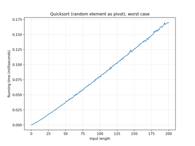
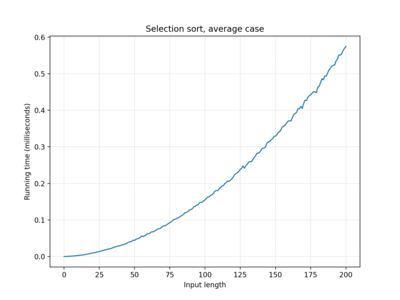
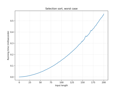
Sorting algorithms
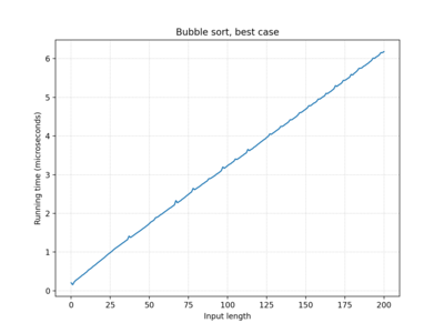
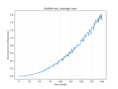
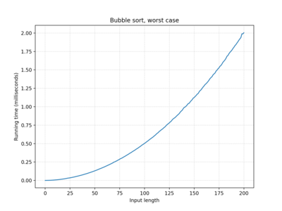
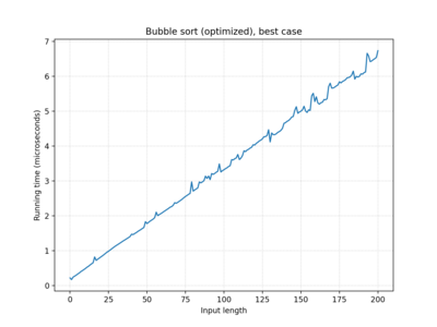
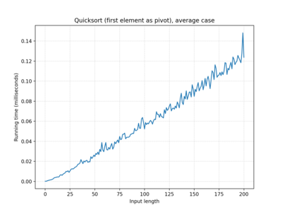
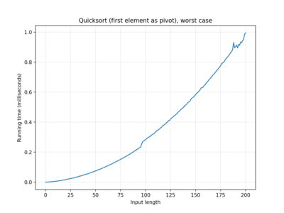
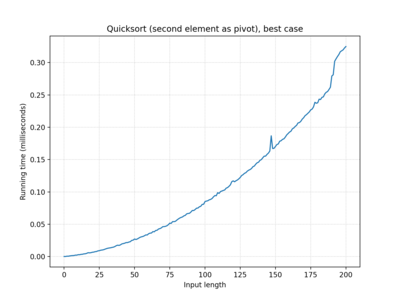
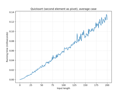
The goals of this "project" include a) familiarizing myself with a few sorting algorithms by examining their (possibly, simplified) implementations and b) studying the way algorithm's running time changes in relation to the length of its input (a.k.a. identifying its time complexity).
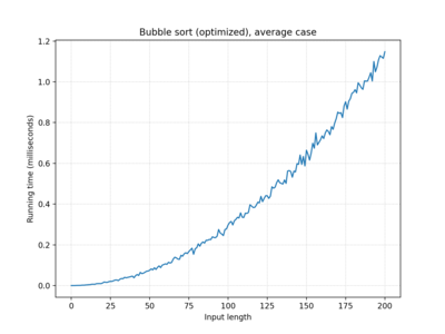
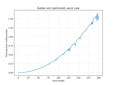
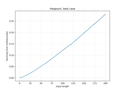
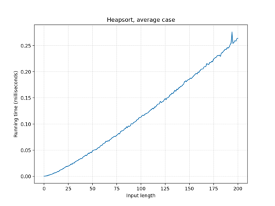
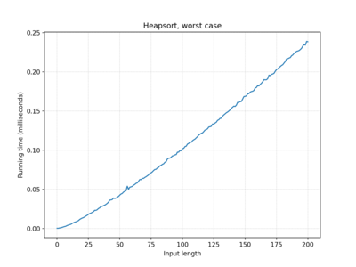
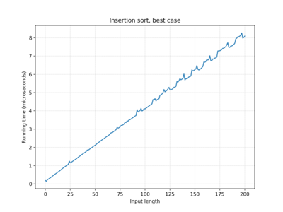
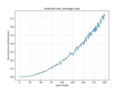
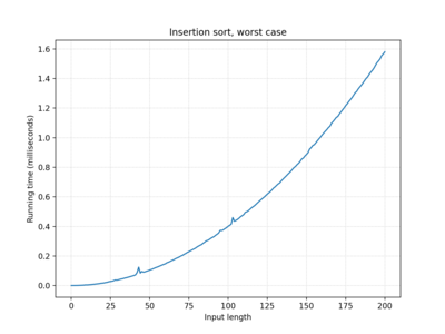
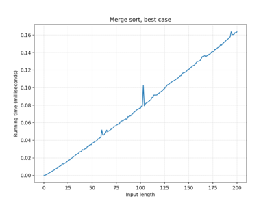
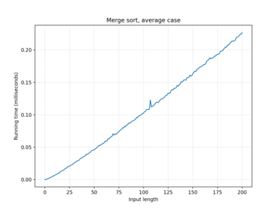
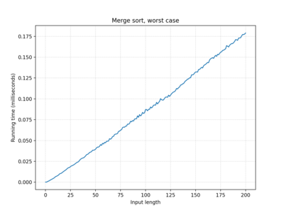
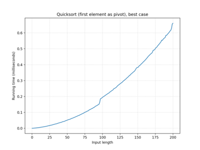
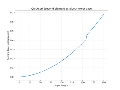
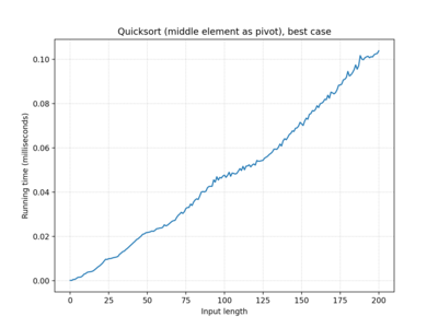
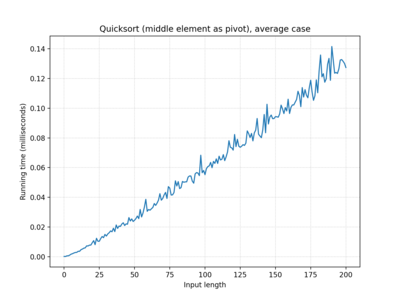
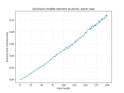
A simple way to visualize the way algorithm's running time changes is to make appropriate measurements and plot them on a nice graph. The results of course are highly dependent on the hardware used, while the graph's look depends on the software used for rendering.
Both the hardware & the software that were used to produce the plots are listed below.
| CPU | Intel Core i7-7500U |
|---|---|
| OS | Linux 6.6 |
| CPython | 3.11.6 |
| matplotlib | 3.8.2 |
The table & plots below are just an attempt to nicely lay out the
data generated using the code from the project repository's master
branch.
Visit https://github.com/egor-tensin/sorting-algorithms for more details.
Each of the implemented algorithms was provided with three input sequences:
- a list of n consecutive numbers sorted in ascending order,
- … in descending order,
- … in random order.
Use the table below to quickly navigate to the plots for the corresponding algorithm.
| Algorithm | Complexity | ||
|---|---|---|---|
| Best | Average | Worst | |
| Bubble sort | O(n) | O(n2) | O(n2) |
| … "optimized" | O(n) | O(n2) | O(n2) |
| Heapsort | O(n log n) | O(n log n) | O(n log n) |
| Insertion sort | O(n) | O(n2) | O(n2) |
| Merge sort | O(n log n) | O(n log n) | O(n log n) |
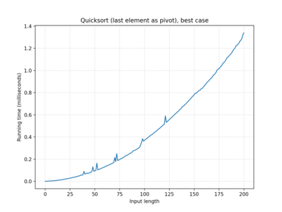
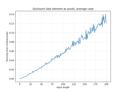
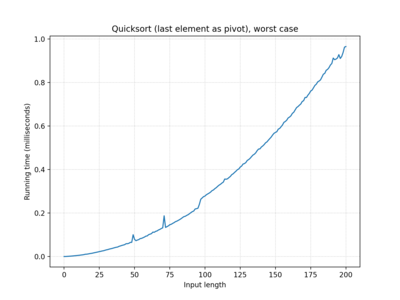
| Quicksort (first element as pivot) | O(n2) | O(n log n) | O(n2) |
| … second element… | O(n2) | O(n log n) | O(n2) |
| … middle element… | O(n log n) | O(n log n) | O(n log n) |
| … last element… | O(n2) | O(n log n) | O(n2) |
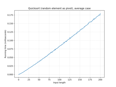
| … random element… | O(n log n) | O(n log n) | O(n log n) |
| Selection sort | O(n2) | O(n2) | O(n2) |
